
A practical overview on probability distributions
A short definition of probability
We can define the probability of a given event by evaluating, in previous observations, the incidence of the same event under circumstances that are as similar as possible to the circumstances we are observing [this is the frequentistic definition of probability, and is based on the relative frequency of an observed event, observed in previous circumstances (1)]. In other words, probability describes the possibility of an event to occur given a series of circumstances (or under a series of pre-event factors). It is a form of inference, a way to predict what may happen, based on what happened before under the same (never exactly the same) circumstances. Probability can vary from 0 (our expected event was never observed, and should never happen) to 1 (or 100%, the event is almost sure). It is described by the following formula: if X = probability of a given x event (Eq. [1]):

This is one of the three axioms of probability, as described by Kolmogorov (2):
- If under some circumstances, a given number of events (E) could verify (E1, E2, E3, …, En), the probability (P) of any E is always more than zero;
- The sum of the probabilities of
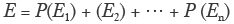 is 100%;
 - If E1 and E3 are two possible events, the probability that one or the other could happen P (E1 or E3) is equal to the sum of the probability of E1 and the probability of E3 (Eq. [2]):
 is 100%;
Probability could be described by a formula, a graph, in which each event is linked to its probability. This kind of description of probability is called probability distribution.
Binomial distribution
A classic example of probability distribution is the binomial distribution. It is the representation of the probability when only two events may happen, that are mutually exclusive. The typical example is when you toss a coin. You can only have two results. In this case, the probability is 50% for both events. However, binomial distribution may describe also two events that are mutually exclusive but are not equally possible (for instance that a newborn baby will be left-handed or right-handed). The probability that x individuals present a given characteristic, p, that is mutually exclusive of another one, called q, depends on the possible number of combinations of x individuals within the population, called C. If my population is composed of five5 individuals, that can be p or q, I have ten possible combinations of, for instance, three individuals with p is (Eq. [3]):
pppqq, pqqpp, ppqpq, ppqqp, pqpqpq, qpppq, qpqpp, qppqp, qqppp

Then p3q2 will be multiplied for the number of combinations (ten times).
If, in experimental population, I had a big number of individuals (n), the number of combinations of x individuals within the population will be (Eq. [4]):
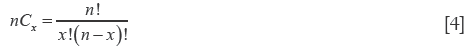
Therefore, the probability that a group of x individuals within the population of n individuals presents the characteristic p, that excludes q, will be described by the following formula (Eq. [5]):

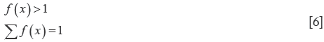
that describes the binomial distribution. It follows the Kolmogorow’s rules (Eq. [6]:
In a given population, 30% of the people are left-handed. If we select ten individuals from this population, what is the probability that four out of ten individuals are left handed?
We can apply the binomial distribution, since we suppose that a person may be either left-handed or right-handed.
Se we can use our formula (Eq. [7]):

Poisson distribution
Another important distribution of probability is the Poisson distribution. It is useful to describe the probability that a given event can happen within a given period (for instance, how many thoracic traumas could need the involvement of the thoracic surgeon in a day, or a week, etc.). The events that may be described by this distribution have the following characteristics:
- The events are independent from one another;
- Within a given interval the event may present from 0 to infinite times;
- The probability of an event to happen increases when the period of observation is longer.
To predict the probability, I must know how the events behave (this data comes from previous, or historical, observations of the same event before the time I am trying to perform my analysis). This parameter, that is a mean of the events in a given interval, as derived from previous observations, is called λ.
The Poisson distribution follows the following formula (Eq. [8]):
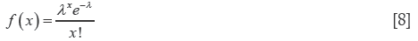
where the number e is an important mathematical constant that is the base of the natural logarithm. It is approximately equal to 2.71828.
For example, the distribution of major thoracic traumas needing intensive care unit (ICU) recovery during a month in the last three years in a Third Level Trauma Center follows a Poisson distribution, were λ=2.75. In a future period of one month, what is the probability to have three patients with major thoracic trauma in ICU? (Eq. [9]):

Therefore, the probability is 22.1%.
The binomial distribution refers only to discrete variables (that present a limited number of values within a given interval). However, in nature, many variables may present an infinite distribution of values, within a given interval. These are called continuous variables (3).
Distributions of continuous variables
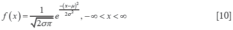
An example of continuous variable is the systolic blood pressure. Within a given cohort of systolic blood pressure can be presented as in Figure 1. Each single histogram length represents an interval of the measure of interest between two intervals on the x-axis, while the histogram height represents the number of measured values within the interval. When the number of observation becomes very large (tends to infinite) and the length of the histogram becomes narrower (tends to 0), the above representation becomes more similar to a curved line (Figure 2). This curve describes the distribution of probability, f (density of probability) for any given value of x, the continuous variable. The area under the curve is equal to 1 (100% of probability). We can now assume that the value of our continuous variable X depends on a very large number of other factors (in many cases beyond our possibility of direct analysis), the probability distribution of X becomes similar to a particular form of distribution, called normal distribution or Gauss distribution. The aforementioned concept is the famous Central Limit Theorem. The normal distribution represents a very important distribution of probability because f, that is the distribution of probability of our variables, can be represented by only two parameters:


- µ = mean;
- σ = standard deviation.
The mean is a so-called measure of central tendency (it represents the more central value of our curve), while the standard deviation represents how dispersed are the values of probability around the central value (is a measure of dispersion).
- The main characteristics of this distribution are:
- It is symmetric around the µ;
- The area under the curve is 1;
If we consider the area under the curve between µ ± σ, this area will cover 68% of all the possible values of X, while the area between µ ± 2σ, it will cover 95% of all the values.
The two parameters of the distribution are linked in the formula (Eq. [10]):
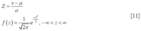
For µ = 0, and σ = 1, the curve is called standardized normal distribution. All the possible normal distributions of x may be “normalized” by defining a derived variable called z. (Eq. [11]):
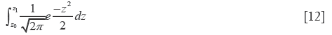
To calculate the probability that our variable falls within a given interval, for instance z0 and z1, we should calculate the following definite integral calculus (Eq. [12]):
Fortunately, for the standard normalized distribution of z every possible interval has been tabulated.
In a given population of adult men, the mean weight is 70 kg, with a standard deviation of 3 kg. What is the probability that a randomly selected individual from this population would have a weight of 65 kg or less?
To “normalize” our distribution, we should calculate the value of z (Eq. [13]):

Then, we should calculate the area under the curve (Eq. [14]):
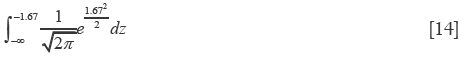
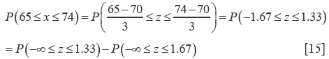
The value of our interval has been already calculated and tabulated [the tables can be easily found in any text of statistics or in the web (4)]. Our probability is 0.0475 (4.75%). We may also calculate the probability to find, within the same population, someone whose weight is between 65 and 74 kg. This probability can be seen as the difference of distribution between those whose weight is 74 kg or less and those whose weight is 65 kg or less: (Eq. [15]):
We already know that (Eq. [16]):

In the table we can find also the value for (Eq. [17]):

Our probability is (Eq. [18]):

Conclusions
The probability distributions are a common way to describe, and possibly predict, the probability of an event. The main point is to define the character of the variables whose behaviour we are trying to describe, trough probability (discrete or continuous). The identification of the right category will allow a proper application of a model (for instance, the standardized normal distribution) that would easily predict the probability of a given event.
Acknowledgements
Disclosure: The authors declare no conflict of interest.
References
- Daniel WW. eds. Biostatistics: a foundation for analysis in the health sciences. New York: John Wiley & Sons, 1995.
- Kolmogorov AN. eds. Foundations of Theory of Probability. Oxford: Chelsea Publishing, 1950.
- Lim E. Basic statistics (the fundamental concepts). J Thorac Dis 2014;6:1875-8. [PubMed]
- Standard Normal Distribution Table. Available online: http://www.mathsisfun.com/data/standard-normal-distribution-table.html

