
A general introduction to adjustment for multiple comparisons
Introduction
The statistical inference would be a critical step of experimental researches, such as in medicine, molecular biology, bioinformatics, agricultural science, etc. It is well acceptable that an appropriate significance level α, such as 0.05 or 0.01, is pre-specified to guarantee the probability of incorrectly rejecting a single test of null hypothesis (H0) no larger than α. However, there are many situations where more than one or even a large number of hypotheses are simultaneously tested, which is referred to as multiple comparisons (1). For example, it is common in clinical trials to simultaneously compare the therapeutic effects of more than one dose levels of a new drug in comparison with standard treatment. A similar problem is to evaluate whether there is difference between treatment and control groups according to multiple outcome measurements. Due to rapid advances of high-throughput sequencing technologies, it is also common to simultaneously determine differential expression among tens of thousands of genes.
The statistical probability of incorrectly rejecting a true H0 will significantly inflate along with the increased number of simultaneously tested hypotheses. In the most general case where all H0 are supposed to be true and also independent with each other, the statistical inference of committing at least one incorrect rejection will become inevitable even when 100 hypotheses are individually tested at significance level α=0.05 (Figure 1). In other words, if we simultaneously test 10,000 true and independent hypotheses, it will incorrectly reject 500 hypotheses and declare them significant at α=0.05. Of course, estimation of error rate would become more complex when hypotheses are correlated in fact and not all of them are true. Therefore, it is obvious that the proper adjustment of statistical inference is required for multiple comparisons (2). In the present paper, we provide a brief introduction to multiple comparisons about the mathematical framework, general concepts and the wildly used adjustment methods.

Mathematical framework
For a simultaneous testing of m hypotheses, the possible outcomes are listed in Table 1. Let’s suppose that the number of true H0 is m0, which is an unobservable random variable (0≤m0≤m). After performing statistical inferences we totally found R H0 being rejected and declared significant at the pre-specified significance level; and herein R is an observable random variable (0≤R≤m). Among the statistically rejected hypotheses of R, when R>0, we suppose that there are U H0 that have been incorrectly rejected. Similar to m0,

Full table
Type I and II errors
For the statistical inference of multiple comparisons, it would commit two main types of errors that are denoted as Type I and Type II errors, respectively. The Type I error is that we incorrectly reject a true H0, whereas Type II error is referred to a false negative. Because the exact numbers of Type I and Type II errors are unobservable (as denoted in Table 1), we would intend to control the probability of committing these errors under acceptable levels. In general, the controlled probabilities of committing Type I and Type II errors are negatively correlated, for which therefore we must determine an appropriate trade-off according to various experimental properties and study purposes. If a significant conclusion has important practical consequence, such as to declare an effective new treatment, we would control Type I error more rigorously. On the other hand, we should avoid committing too many Type II errors when it intends to obtain primary candidates for further investigation, which is very common in studies of genomics. Here, we specially address the controlling of Type I error because it considerably increases for multiple comparisons.
Adjusted P value or significance level
In statistical inference, a probability value (namely P value) is directly or indirectly computed for each hypothesis and then compared with the pre-specified significance level α for determining this H0 should be rejected or not (3). Therefore, there are two ways for adjusting the statistical inference of multiple comparisons. First, it could directly adjust the observed P value for each hypothesis and keep the pre-specified significance level α unchanging; and this is herein referred to as the adjusted P value. Second, an adjusted cut-off corresponding to the initially pre-specified α could be also computationally determined and then compared with the observed P value for statistical inference. In general, the adjusted P value is more convenient because in which the perceptible significance level is employed. However, it would be difficult or impossible to accurately compute the adjusted P value in some situations.
Measures accounting for Type I error
According to possible outcomes of multiple comparisons (Table 1), all efforts would be paid to the control of variable U, for which therefore various statistical measures have been proposed to account (4). Certainly, each of these measures has differential applications with respective strengths and weaknesses.
A simple and straightforward measurement is the expected proportion of variable U among all simultaneously tested hypotheses of m, which is referred to as the per-comparison error rate (PCER):
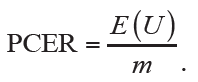
If each hypothesis is separately tested at significance level α, PCER will be equal to αwhen all H0 are true and independent with each other. Obviously, it becomes PCER=αm0/m≤α when not all H0 are true in fact. However, control of PCER would be less efficient because we would obtain at least one false positive at significance level α=0.05 when 20 true H0 are simultaneously tested.
In practical applications, it is more reasonable to jointly consider all hypotheses as a family for controlling Type I error; and therefore the most stringent criterion is to guarantee that not any H0 is incorrectly rejected. Accordingly, the measure of familywise error rate (FWER) is introduced and defined as the probability of incorrectly rejecting at least one H0:
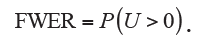
The control of FWER has been widely used especially when only a few or at most several tens of hypotheses are simultaneously tested. However, FWER is believed to be too conservative in cases that the number of simultaneously tested hypotheses reaches several hundreds or thousands.
Another popular measure for controlling Type I error of multiple comparisons is the false discovery rate (FDR), which is defined as the expected proportion of incorrectly rejected H0 among all rejections:
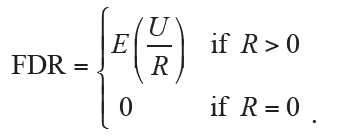
Therefore, FDR allows the occurrence of Type I errors under a reasonable proportion by taking the total number of rejections into consideration. An obvious advantage of FDR controlling is the greatly improved power of statistical inference, which would be useful when a large number of hypotheses are simultaneously tested.
Common methods for adjustment
Suppose that there are m hypotheses of H1, …, Hmbeing simultaneously tested, which correspond to the initially computed P values of p1, …, pm. Accordingly, the adjusted P values of multiple comparisons are denoted as  , …,
, …,  . The pre-specified and adjusted significance levels are further denoted as α and α’, respectively. Furthermore, we assume that all hypotheses are ordered as H(1), …, H(m)according to their observed P values of
  ; and the associated P values and significance level are denoted as
  ,
,  and
and  for the
  ordered hypothesis of H(i). We here provide an illustrative example for demonstrating differences among various adjustment methods. Let m=6 and α=0.05; and the initially computed P values corresponding to six hypotheses are p1=0.1025, p2=0.0085, p3=0.0045, p4=0.0658, p5=0.0201 and p6=0.0304, respectively.
Bonferroni adjustment
Bonferroni adjustment is one of the most commonly used approaches for multiple comparisons (5). This method tries to control FWER in a very stringent criterion and compute the adjusted P values by directly multiplying the number of simultaneously tested hypotheses (m):
Equivalently, we could let the observed P values unchanging and directly adjust the significance level as  . For our illustrative example the adjusted P values are compared with the pre-specified significance level α=0.05, and the statistical conclusion is obviously altered before and after adjustment (Figure 2). Bonferroni adjustment has been well acknowledged to be much conservative especially when there are a large number of hypotheses being simultaneously tested and/or hypotheses are highly correlated.

Differences of the adjusted P values among various methods. The dashed horizontal line denotes the pre-specified significance level.
Holm adjustment
On the basis of Bonferroni method, Holm adjustment was subsequently proposed with less conservative character (6). Holm method, in a stepwise way, computes the significance levels depending on the P value based rank of hypotheses. For the  ordered hypothesis H(i), the specifically adjusted significance level is computed:
The observed P value p(i) of hypothesis H(i) is then compared with its corresponding  for statistical inference; and each hypothesis will be tested in order from the smallest to largest P values (H(1), …, H(m)). The comparison will immediately stop when the first
  is observed (i=1,…,m) and hence all remaining hypotheses of H(j) (j=i,…,m)are directly declared non-significant without requiring individual comparison (Figure 3). Alternatively, it could directly compute the adjusted P value for each hypothesis and produce same conclusion (Figure 2).

Hochberg adjustment
Similar to Holm method, Hochberg adjustment employs same formula for computing the associated significance levels (7). Therefore, the specifically adjusted significance level for ith ordered hypothesis H(i) is also computed:
However, Hochberg method conducts statistical inference of hypothesis by starting with the largest P value (H(m), …, H(1)). When we first observe  for hypothesis H(i)(i=m,…,1), the comparison stops and then concludes that the hypotheses of H(j)(j=i,…,1) will be rejected at significance level α. The adjusted P values of Hochberg method are shown in Figure 2. It is also known that Hochberg adjustment is more powerful than Holm method.
Hommel adjustment
Simes (1986) modified Bonferroni method and proposed a global test of m hypotheses (8). Let H={ H(1), …, H(m)} be the global intersection hypothesis, H will be rejected if  for any i=1,..., m. However, Simes global test could not be used for assessing the individual hypothesis Hi. Therefore, Hommel (1988) extended Simes’ method for testing individual Hi (9). Let an index of
  be the size of the largest subset of m hypotheses for which Simes test is not significant. All Hi (i=1,…,m) are rejected if j does not exist, otherwise reject all Hi with pi≤α/j. Although straightforward explanation for computing the adjusted P values of Hommel method would be not easy, this task could be conveniently performed by computer tools, such as the p.adjust() function in R stats package (http://cran.r-project.org).
Benjamini-Hochberg (BH) adjustment
In contrast to the strong control of FWER, Benjamini and Hochberg [1995] introduced a method for controlling FDR, which is herein termed BH adjustment (10). Let be the pre-specified upper bound of FDR (e.g., q=0.05), the first step is to compute index:
If k does not exist, reject no hypothesis, otherwise reject hypothesis of Hi (i=1,…,k). BH method starts with comparing H(i) from the largest to smallest P value (i=m,…,1). The FDR-based control is less stringent with the increased gain in power (Figure 2) and has been widely used in cases where a large number of hypotheses are simultaneously tested.
Benjamini and Yekutieli (BY) adjustment
Similar to BH method, a more conservative adjustment was further proposed for controlling FDR by Benjamini and Yekutieli [2001], and this method is also termed BY adjustment (11). Let again q be the pre-specified upper bound of FDR, the index k is computed as:
If does not exist, reject no hypothesis, otherwise reject hypothesis of Hi (i=1,…,k). BY method could address the dependency of hypotheses with increased advantages.
Conclusions
Although substantial literature has been published for addressing the increased Type I errors of multiple comparisons during the past decades, many researchers are puzzling in selecting an appropriate adjustment method. Therefore, it would be helpful for providing a straightforward overview on the adjustment for multiple comparisons to researchers who don’t have good background in statistics. Of course, there are many theoretical topics and methodological issues having not been addressed yet in the present paper, such as resampling-based adjustment methods, choice of significance level α, and specific concerns for genomics data. It is also beyond the scope of this paper to discuss the sophisticated mathematical issues in this filed.
Acknowledgements
None.
Footnote
Conflicts of Interest: The authors have no conflicts of interest to declare.
References
- Hsu JC. Multiple comparisons: theory and methods. London: Chapman & Hall: CRC Press, 1996.
- Bender R, Lange S. Adjusting for multiple testing—when and how? J Clin Epidemiol 2001;54:343-9. [Crossref] [PubMed]
- Thiese MS, Ronna B, Ott U. P value interpretations and considerations. J Thorac Dis 2016;8:E928-E931. [Crossref] [PubMed]
- Farcomeni A. A review of modern multiple hypothesis testing, with particular attention to the false discovery proportion. Stat Methods Med Res 2008;17:347-88. [Crossref] [PubMed]
- Bland JM, Altman DG. Multiple significance tests: the Bonferroni method. BMJ 1995;310:170. [Crossref] [PubMed]
- Holm M. A simple sequentially rejective multiple test procedure. Scand J Statist 1979;6:65-70.
- Hochberg Y. A sharper Bonferroni procedure for multiple tests of significance. Biometrika 1988;75:800-2. [Crossref]
- Simes RJ. An improved Bonferroni procedure for multiple tests of significance. Biometrika 1986;73:751-4. [Crossref]
- Hommel G. A stagewise rejective multiple test procedure based on a modified Bonferroni test. Biometrika 1988;75:383-6. [Crossref]
- Benjamini Y, Hochberg Y. Controlling the false discovery rate: a practical and powerful approach to multiple testing. J R Stat Soc Series B Stat Methodol 1995;57:289-300.
- Benjamini Y, Yekutieli D. The control of the false discovery rate in multiple testing under dependency. Ann Stat 2001;29:1165-88.

