
Basic statistics with Microsoft Excel: a review
Introduction
The value of a scientific study is recognized by the community only if it is supported by numerical evidence that warrants the validity. In this sense, statistical analysis plays a central role. The term “Statistics” was introduced in the seventeenth century with the meaning of “science of the state” (1), which aims to gather and sort information to the public administration regarding: size and composition of the population, migration, demographic changes, birth and mortality tables, data on businesses, crops, the distribution of wealth, education and health. The first step of statistical work is the collection of data, which, if well organized, saves effort in subsequent operations and allows the correct setting for the analysis. The mathematical concepts presented in this discussion represent the basis of the statistical models used in platforms of spreadsheets. The spreadsheet arises from the need to modify, through a specific “software”, a certain amount of data with the ability to automatically update the results deriving from the analysis of these without reprogramming entire columns of calculation. This makes it particularly easy to insert and/or modify data previously collected within certain sectors such as occurs in research studies. The software that use spreadsheets are fundamental in different scientific fields but require an understanding of basic mathematical concepts that regulate the operation. The purpose of the study was to provide the necessary statistical information in order to facilitate access to the vast potential of Microsoft Excel correctly.
Arithmetic mean, median and percentiles
The first step of statistical work is the collection of data, which, if well organized, save effort in subsequent operations and allows the correct setting of the analysis. Three are the key points (2,3):
- Statistical units defined as the minimum unit of which the data are collected;
- The population is defined as the whole of the statistical units under study;
- The font is defined as the properties that are being surveyed. Characters can be qualitative or quantitative.
The statistical variables can be qualitative, if they express an individual quality (i.e., color and shape of leaves and fruit). A qualitative variable is not measured, but classified into categories based on the manner in which it is presented (smooth or wrinkled peas, green or yellow). On the other hand, there are quantitative variables, which can be measured on a discrete scale. The quantitative traits can be expressed numerically and are divided into discrete and continuous. The discrete characters, such as the number of pupils in a class, or of goals scored in a football match, can only take on certain values, usually integers. The continuous characters, such as weights, heights and, more generally, the quantities that can be measured, can assume any real value in a given interval (although usually it takes finite decimal numbers). The statistics can be divided into two areas of application:
- Descriptive, its goal is to obtain a set of data in tables and graphs (too numerous to be individually examined) some significant information for the problem studied;
- Inferential, its goal is to provide methods that are used to learn from experience, that is to build models to go from particular cases to the general case. In inferential statistics or inductive, also they use techniques of probability calculations.

Qualitative information can be quantified using the following indices:

Mean
It is possible to obtain various averages from a sequence of data which have different names (4). Basically, an average is a value suitably chosen between the minimum and the maximum of the data. In all cases, the mean is a number that summarizes many, and allows a unified vision, obviously hiding the multiplicity of data from which it derives. Thus, the average income of Italian families is a unique value, useful for making comparisons with other countries or past periods, but does not show that incomes are very different and many families are below the survival threshold, while others have assets in large quantities. The mean height allows us to say that the Swedes are, on average, taller than Italians, but does not reveal that many Italians are taller than many Swedes. We will look at the following mean: mode, median, arithmetic mean, quadratic mean, geometric mean and harmonic mean. Let us then examine the fixed mean, those averages that take into account all data, regardless of their order. By varying, even slightly, even one of the data, they vary continuously and without jumps. The fixed average may only be used for numeric data. In statistics, they are usually distinguished two types of mean: (I) mean calculation (or stationary), which satisfies a condition of invariance and is calculated taking into account all values of the distribution; (II) mean of position (or loose), calculated taking into account only of some values. Of course, the choice of the type of media to be used depends on the problem that is being examined. We study four types of medium calculation (arithmetic, geometric, quadratic, and harmonic) and two types of medium position (median, mode or normal value).
The arithmetic mean
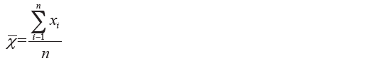
Given n values X1, X2, ..., Xn is called arithmetic mean (or simply mean) the value that is obtained by dividing the sum by the number n; denoting by x the average, in the formula, we have:
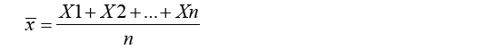
in general:
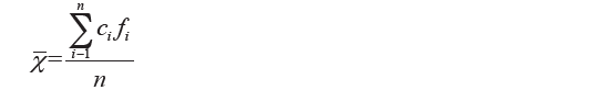
The mean properties are: (I) internalities; (II) barycentric interpolation; (III) equivariance compared to linear transformations; (IV) associative; (V) minimization of the sum of the quadratic deviations. If a collective is divided into “G” disjoint subsets, then the mean overall arithmetic can be achieved as a weighted mean of the mean of subsets with weights equal to their number. The arithmetic mean, by far the best known and most used of the mean, is the most reliable value in the following two cases: (I) when performing different measurements of the same magnitude; (II) when measuring the typical value in a homogeneous population. In the first case, when measuring a physical quantity with a tool several times you do not always get the same result. This is due to several factors: the fact that, by operating at a later time, the environmental conditions may have changed (temperature, humidity, atmospheric pressure) which influence the quantity to be measured and the instrument, the method of use of the instrument, uncertainties in reading scales, and so on. Precisely for this reason, when you want to know the precise measurement of a magnitude, this can be shown by performing different measurements. If the differences between the obtained measures are due to accidental errors, the arithmetic average of the measurements is the most reliable value of the measure of the greatness. In the second case, when reproducing metal pieces with a mold these should all have the same weight. But if you weigh the pieces produced, the weights will be different, as a result of measurement errors, as mentioned in the previous point, as to production errors (the metallic material is not perfectly homogeneous, the various pieces have never form identical, the operation of the mold is influenced by environmental factors that vary over time, etc.). It gives the typical weight that each piece should have (according to the ideal model derived from the mold) the arithmetic average of the weights obtained can be shown. However, it may be greatly affected by extreme values in the case in which the distribution is not symmetric. Often, instead of the simple arithmetic average, using the weighted average: no values assigned to X1, X2, ..., Xn the weights p1, p2, .., pn proportion to the importance that we attribute to them, the arithmetic mean is weighted:
Geometric mean and its properties
If the values are all positive and not zero you can calculate the geometric mean. It defines the geometric mean of the values x1, x2, …, xn, the G number that replaced the xi values bring no changes to their product:

from which:

that is the simple geometric mean.
If xi yi values with frequencies or weights, you have:

then:

in which:
is the weighted geometric mean. Obviously, you cannot calculate the geometric mean if one of the values is zero because the product would be zero for any value taken from others. Furthermore, xi cannot be negative. For the calculation of the geometric average using formulas obtained from the previous two definitions using logarithms (in any base) that turn them into an arithmetical average, respectively, simple or weighted. Taking logarithm yields:
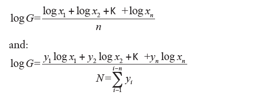
Then, the logarithm of the geometric average (simple or weighted) is the arithmetic average (simple or weighted) of the logarithms of the statistical variable values. It uses the geometric average when it makes sense to multiply together the statistical data. You must calculate the geometric average, and not the arithmetic average, for example, to determine the average rate of increase or decrease in prices, or the growth rate of a population. It uses the geometric average when the data varies in geometric progression. Even the geometric average (simple or weighted), enjoys certain properties including.
First property
By multiplying (or dividing) all xi values for a same amount h, greater than zero, the geometric average is multiplied (or divided) for that quantity:
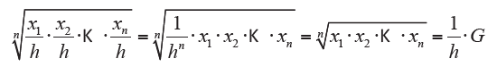
This property is very useful to simplify the calculations.
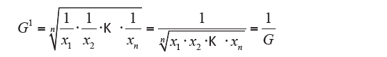
Second property
The reciprocal of the geometric average is equal to the geometric average of the reciprocal of the values:
Quadratic mean
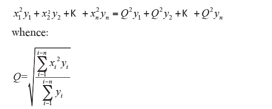
If we assume function as the sum of the quadratics of the values, indicating with Q the quadratic mean, we have, for the usual definition

practically:
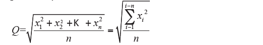
which it is the simple quadratic mean (also denoted by M2). If the values have different frequencies yi you have:
which is the weighted quadratic mean. The quadratic mean (simple or weighted) is equal to the root mean square of the arithmetic mean (simple or weighted) of the quadratics of the data values. Among the considered medium, the quadratic mean is the one that has higher value and is the most influenced by very small or very large values of the distribution; the root mean square is therefore used to highlight the existence of values that differ a lot from the central values. It also uses the quadratic mean when it has an interest to calculate an average value of available surface
Harmonic mean
The harmonic average is the value which when replaced leaves unchanged the sum of the reciprocals, in other words:
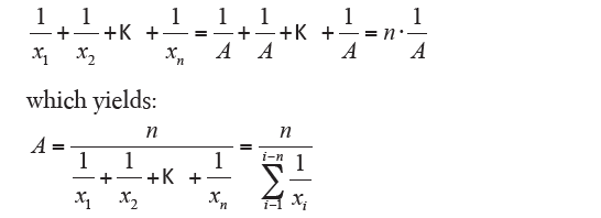
that is the simple harmonic mean. If the values have different frequencies yi, with analogous procedure it goes on to the formula:
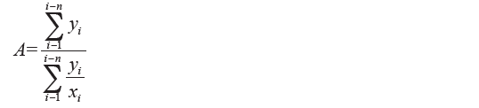
that expresses the weighted harmonic mean.
The harmonic mean, simple or weighted, is equal to the reciprocal of the arithmetic mean, simple or weighted, of the reciprocals. The harmonic mean is applied when it makes sense to calculate the reciprocal of the data. The harmonic mean can also be applied also to discover the mean speed as a harmonic mean speed, since the reciprocal of a speed represents the time required to cover a unity of space. Among the four averages calculation examined, there is the following relationship:

The equal sign is necessary only in the case where the data are all equal among themselves and therefore equal to any average. The arithmetic, quadratic and harmonic mean, are special cases of the general formula:
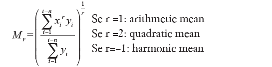
(with regard to the geometric mean denoted by M0, it falls if r tends to zero power averages).
Mode
The mode is the observation that occurs most frequently.
The distribution of frequency of the model class is represented as follows:

Median
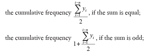
The median is an average of position and represents the central value of the distribution when the data are sorted. Precisely: let x1, x2, ..., xn values sorted in a non-decreasing sense, it is called median Me when the value is not less than half of the values and not more than the other half. Sorted values, if the number of terms n is odd, the median is just the central value; if n is even, it is taken as the median semi-sum of the two central values. The above procedure applies to the series. For frequency distributions with discrete values, the data are generally already ordained; it is then necessary to calculate the cumulative absolute frequencies, which are obtained by associating to each value from the sum of the respective frequency with all those which precede it, and determine which value corresponds:
this value is the median. If the data is grouped into classes, the median class is determined by using the absolute cumulative frequency. To obtain the exact median value, linear interpolation between the two extreme values of the class in which the median falls is applied, assuming that the frequencies are distributed at regular intervals in the class. For the approximate calculation in this case it is useful to make use of the polygonal plots of cumulative relative frequencies. The median is not influenced by the distribution of the extreme values, so even if the extreme classes, in the case of continuous distribution, are open, there is no need to close them. In addition, if the distribution is highly asymmetrical, the median value is more appropriate than the arithmetic mean to express a synthetic value of the distribution. A feature of the median property is as follows: the median minimizes the sum of the absolute values of the deviations, in other words the sum of the absolute values of deviations from the median, and is not higher (i.e., less than or equal to) the sum of the discard values from any other value. Next to the median the first and third quartile are considered.
Percentiles
Percentiles are a family of indicators similar to the median. They are thus called because a percentile bisects the normal population so as to leave a certain amount of terms to its left and the remaining amount to its right. The percentile is 99, for example, the first percentile bisects the population so as to leave on the left 1% of the terms and to the right the remaining 99%. Similarly, the eightieth percentile bisects the population so as to leave on the left 80% of the terms and the remaining 20% to the right. In particular: (I) p-th quantile/100p percentile is considered np; (II) if np is not a whole number, k is considered the next whole number and the p-th quantile is xk; (III) if np = k is a whole, the p-th quantile is (xk + xk + 1)/2; (IV) Q1 = first quartile = 25th percentile; (V) Q2 = second quartile = 50th percentile = median; (VI) Q3 = third quartile = 75th percentile.
How to choose a mean
A synthetic value can be calculated in various ways (5). Some mean values satisfy a condition of invariance of a global value, namely: the mean leaves the sum of terms unchanged, the geometric mean makes no changes to the product, the root mean square leaves unchanged the sum of the quadratics of the terms and the harmonic mean the sum of the reciprocals of the terms. You use the arithmetic mean to determine a value that expresses a concept of equitable distribution when, for example, you want to determine an average of the costs, consumption, income, temperature. It also applies the arithmetic mean, for the properties of its waste, to determine the precise value of a series of measures, provided that the measurement errors are accidental and not systematic (in practice due to the instruments); the arithmetic mean also applies if your data follow one another in arithmetic progression. The geometric mean is used to determine the average rate of increase (or decrease) of a phenomenon, the average interest rate of more rate in compound interest, or to determine an average exchange rates in the money. The geometric average is used even when the data are followed in geometric progression. The quadratic mean is applied when you have to eliminate the influence of the signs and when you have to highlight the existence in the distribution of very large or very small values. The harmonic mean is applied when you want to know the average value using the reciprocal values of another character, such as the purchasing power of the currency. The mode or the normal value of a frequency distribution is important when it is necessary to know the value that has is most probable to show up. The median value is the central value of the distribution and is independent of strong differences between the data. You cannot give a general rule for choosing the type of media, but you have to calculate more than an average value and choose the most adequate for the resolving the problem at hand. The medium which is used most frequently in practice are the arithmetic mean, the median and, in the case of frequency distributions, the modal value.
The dispersion index (6)
 Range
Range
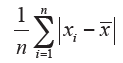 Average absolute difference
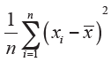 Mean of squares of deviations
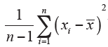 Variance
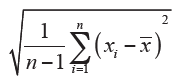 Standard deviation
The shape index [6]
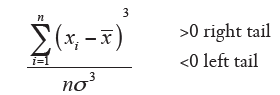
Asymmetry index (Skewness)
Kurtosis measures how much the pointed distribution
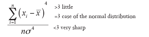
In many the coefficient software. kurtosis is compared with the value 0.
Frequencies and frequency distributions
In statistics having to do with a large number of data, it is convenient to consider the frequencies of the experimental units (7): the absolute frequency is no more than the number of individuals who exhibit a certain extent (for a quantitative character) or a certain mode (for a qualitative character). If we are dealing with quantitative variables on a continuous scale, before calculating the frequencies it is convenient to split the range of measures in a number of frequency classes.
Relative frequencies
By dividing the absolute frequency by the total number of statistical units we get the so-called relative frequencies. The advantage with respect to the absolute frequencies consist in the comparison of frequency distributions based on different numbers of statistical units. It defines: (I) the relative frequency of a mode, the frequency of the uniform mode to the total number of frequencies; (II) the relative intensity of a mode, the intensity of the divided by the total of the intensity mode.
Accumulating frequencies
The characteristics are as follows: (I) similar to the empirical distribution function; (II) “accumulating” gradually frequencies; (III) “absolute” or “relative”. Those related to coincide with the empirical distribution function at the end of each interval.
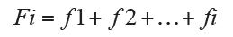
The absolute cumulative frequency Fi is the sum of the absolute frequency relative to Xi mode and absolute frequencies that precede it, then:
The relative cumulative frequency Ri is the sum of the relative frequency corresponding to Xi mode and its associated frequencies that precede it, then:

Graphical representations and histograms
Graphs in tapes and columns
The graphs in tapes and columns are the first form of graphical representation and are often used to represent mutable or statistical variables. The data tables are represented by drawing generic rectangles width and length proportional to the frequency or the intensity of the mode. The rectangles can be arranged horizontally (graph tapes) or vertically (in columns graphics).
Graphs in circular sectors
They use the graphs in circular sectors in order to better highlight the subdivision of the phenomenon between the various modes that compose it. The frequency or the total intensity of the phenomenon is represented by the area around the circle, while the areas of each sector represent the frequencies or intensities of the individual modes:
Histograms
Histograms are made up of as many rectangles as there are classes. If all classes have the same amplitude, the rectangles have equal bases and the heights are proportional to the frequencies of the classes. In the presence of classes with different amplitude it is necessary that the heights of the rectangles be proportional to the frequency density, i.e., the frequency divided by the amplitude of the class, in order to maintain proportionality between the areas. There are two types of histograms: (I) for classes of equal amplitude mode (in this case the rectangles have base equal to the width of class and height equal to or proportional to the frequency class); (II) for classes of different amplitude mode (in this case the rectangles have a base equal to the width of the class and the height equal to the frequency density that is given by the ratio between the frequency and the amplitude of class).
Microsoft Excel statistical analysis examples
The Excel program includes a spreadsheet format of contiguous cells to form a grid. Each cell can contain both data and formulas. Structurally, the data can be values such as numbers, dates, times, percentages or texts. The structure of the formulas is constituted by the following string: =FUNCTION (Topic1; Topic2; ...) where the topics can be numbers, text, cell references, formulas, functions separated by punctuation. Types of functions are as follows: (I) average, to calculate the average of a range of cells use the AVERAGE function =AVERAGE (num1; num2; ….); (II) median, to find the median (or middle number), use the MEDIAN function =MEDIAN (num1; num2; …).
t-test
The t-test is used to test the null hypothesis that the means of two populations are equal. On the formulas table click “Insert function”. Selecting t-test, the string “Function topics” appears: (I) Matrix 1, the first data set; (II) Matrix 2, the second data set (must have length as array 1); (III) Tails, the number of tail for the distribution. This can be either as Tail =1 (uses the one-tailed distribution) and as Tail =2 (uses the two-tailed distribution). The type can be an integer that represents the type of t-test. This is either: (I) paired t-test; (II) two-sample equal variance t-tests; (III) two-sample unequal variance t-test. Then you need to click: (I) in the Matrix 1 and select the range (ex A1: A43); (II) in the Matrix 2 and select the range (ex B1: B43); (III) in the tail (insert 1 or 2); d) in the type (insert 1 or 2 or 3).
Conclusions
To date platforms such as Microsoft Excel exist, which simplify the processing and management of data through the use of spreadsheets. We want to emphasize the importance of understanding the meanings of media, median, frequency distribution and all the statistical concepts that anyone who uses a spreadsheet should know. Many errors in data interpretation result from a lack of knowledge of the mathematical bases of statistical concepts. Understanding it minimizes the chances of improper use of computer media and allows you to show more accurate, reliable, and verifiable results.
Acknowledgements
We want to thank Prof. Filomena Tavares for the valuable contribution.
Footnote
Conflicts of Interest: The authors have no conflicts of interest to declare.
References
- Galvani L, Gini C, Giusti U, Statistica. Available online: http://www.treccani.it/enciclopedia/statistica_res-6a8e2a20-8bb7-11dc-8e9d-0016357eee51
- Windish DM, Diener-West M. A clinician-educator's roadmap to choosing and interpreting statistical tests. J Gen Intern Med 2006;21:656-60. [Crossref] [PubMed]
- Landenna G. editor. Fondamenti di statistica descrittiva. Edt Il Mulino, Bologna, 1984.
- Twycross A, Shields L. Statistics made simple. Part 1. Mean, medians and modes. Paediatr Nurs 2004;16:32. [Crossref] [PubMed]
- Rodrigues CF, Lima FJ, Barbosa FT. Importance of using basic statistics adequately in clinical research. Rev Bras Anestesiol 2017. [Epub ahead of print]. [PubMed]
- Twycross A, Shields L. Statistics made simple. Part 2. Standard deviation, variance and range. Paediatr Nurs 2004;16:24. [Crossref] [PubMed]
- Ballatori E. editor. Statistica e metodologia della ricerca. Edt Margiacchi-Galeno, Perugia, 1990.

