Common data manipulations with R in biological researches
Background
R is a computer language initially designed by the statisticians Ross Ihaka and Robert Gentleman in the 1990s and also famous for the excellent facilities on data analysis and visualization (1). Because it is freely available under the GNU General Public License and runs on UNIX, Windows and MacOS platforms, R can be easily extended via packages to provide all kinds of specialized and sophisticated functions (http://www.r-project.org). Tippmann recently reported that there were about 6,000 R packages published by 2015 and 1% or higher of scholarly articles had cited R or R package(s) (2). It is also anticipated that R will continue to grow in popularity due to the increased requirements for analyzing large-scale data especially in biological and agricultural sciences.
Both data analysis and visualization can be easily implemented with R because the developed packages always provide easy-to-use command-line interface to user and also technically supported by the active online communities. In contrast to these advantages, a tiny but important barrier is that almost all R packages require the strictly specified format of data for inputting, which must be prepared by user in advance. According to our experiences, however, the appropriate preparation of data in accordance with R package’s requirements would be a tough and time-consuming process for most if not all of users. In the present paper, we roughly categorize and exemplify common data manipulations with R in biological researches, which would be helpful for preparing original experimental data more efficiently to R packages.
Data structure and sample data
There are several objects for storing data in R, including vector, matrix, list and data frame. Among them data frame would be one of the most common objects because it is able to combine different models of data, such as numeric, character and factor, into a single table and hence closely resembles the real situations in researches. Therefore all data manipulations outlined in the present paper will start with data frame, and it is also beyond our scope for describing various R objects in details.
In R the data frame is a two-dimensional array-like data structure, in which each row always represents one experimental subject and each column corresponds to a variable for storing measurements on all subjects. Each column of data frame could be arbitrary data model, while all columns must be equal in length. Therefore, any missing measurement in data frame must be specified by uniform character. There is a sample spreadsheet of clinical records for 41 diabetic patients, which contains six columns for storing various attributes and blood measures of patient (Table 1). In this table, the top line is column names and each line afterward corresponds to individual patient; the missing value is specified by character of ‘NA’. We herein use this sample data for exemplifying common manipulations in following sections.

Full table
Common data manipulations
In general, common manipulations prior to formal data analysis and visualization using the developed R packages could be roughly categorized into four classes, including (I) preview overall structure of data; (II) transform the existing variable into new column; (III) summarize data based on the specified groups; and (IV) reorganize the structure of data. Both reading and writing data are not included here because they are relatively straightforward and also beyond scope of data manipulation. Therefore, we suppose that the original dataset has been successfully inputted into R, for instance, the variable of ‘dpData’ has been already linked to our sample data.
Overview of data
At the beginning of data analysis and visualization, it is always necessary to preview the overall structure of data, such as organization of variables, number of observations, levels of a factor variable, etc. Three generic functions of head(), str() and summary() could be used for these purposes; and among them the head() compactly demonstrates the first few rows of a data frame, str() displays variable models, and summary() produces statistical summary for each variable.
Transform
Computing and creating new variable
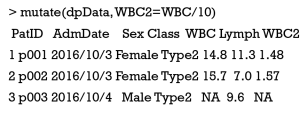
Arbitrary mathematical calculation could be operated on one or more variables, and by which a new variable will be generated and added into the initial data frame. The function of mutate() in plyr package could powerfully perform such task. In the sample data, we simply divide WBC values by 10 for establishing a new column of WBC2.
Recoding factor variable
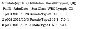
To recode a factor variable is required in some cases, such as in logistic regression analyses with binary variable. A generalized method is to employ the functions of mutate() and ifelse() in tandem; and the ifelse() statement could also be nested when recoding into more than two levels. In the sample data, we recode the Class variable into a new binary variable of C2, in which the value of type 2 corresponds to 1 and others to 0.
Transforming continuous variable(s) into factor variable
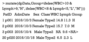
It is able to classify subjects based on one or more continuous variables and then directly transformed into a factor variable, which could also be performed by the functions of mutate() and ifelse() in tandem. In the sample data, we try to classify patients into different groups based on both WBC and Lymph values, from which a new factor variable of Group is generated.
Specifying level order of factor variable
In R the levels of a factor variable would be ordered or unordered, and an ordered factor may have specific meanings for data analysis and visualization. Therefore, it may be necessary in some cases to specify or change level order of factor variable. In the sample data, we use the function of factor() to specify the level order of Sex variable as Male and Female in order:
Also, we could specify level order for a factor variable according to the values of a second variable. In the sample data, we use the function of reorder() to specify the level order of Sex variable according to mean of WBC values for each level.
Renaming levels of factor variable
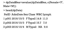
To facilitate data analysis and visualization, it would be helpful to edit the level names for a factor variable, which could be performed by the function of revalue() in plyr package. In the sample data, we simplify the level names of Female and Male for Sex variable into F and M, respectively.
Specifying a date variable
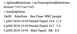
In general, date value is inputted into R as a character or numeric model, which, therefore, must be specified as date model by the function of as.Date() in advance. In the sample data, the AdmDate variable is initially treated as factor model, which is specified as date variable suitable for the following analysis.
Summarize
Summarizing counts or proportions for factor variable
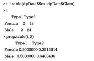
For a factor variable, it is common to summarize the counts or relative proportions for each level into a simple tabulation. A cross-tabulation will be generated when more than one factor variables are jointly used. The generated tabulation and cross-tabulation could be directly transformed into the format of data frame. These tasks could be performed by the functions of table() and prop.table(). In the sample data, we summarize the counts and proportions of patients for two variables of Sex and Class.
Adding margins to rows and/or columns
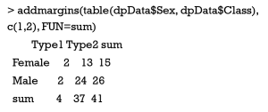
In R the function of addmargins() provides a simple method for summarizing values by rows and/or columns. In the sample data, we summarize the counts and proportions of patients according to both Sex and Class variables and further calculate the sums by both rows and columns.
Computing multiple statistics by groups
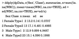
The data aggregation is an important manipulation in data frame, for which a number of methods have been proposed. It is common to compute multiple statistics for a continuous variable based on the specified groups by one or more factor variables. In the sample data, we could use ddply() function in plyr package to compute four statistics, including the number of observation, mean, standard derivation and standard error, for WBC measurements according to both Sex and Class variables.
Computing multiple statistics by columns
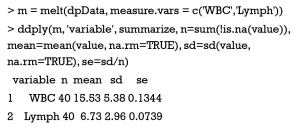
When the summarization of multiple statistics is operated on more than one variables at different columns, an additional step is required before using the ddply() function. That is to use melt() function in reshape2 package to arrange all target variables into a single column. In the sample data, we similarly compute four statistics of the number of observation, mean, standard derivation and standard error for both WBC and Lymph variables.
Reshape
Extracting all columns having the specified model
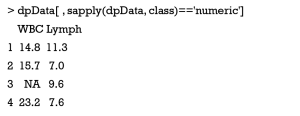
In general, columns of a data frame contain different models of data. Therefore, it is common to extract all columns with the same model, such as numeric and character, and subsequently generate a new data frame. In the sample data, we use sapply() function to extract all numeric columns.
Extracting subset of data frame
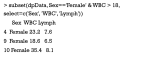
The function of subset() provides a flexible method for extracting a subset of data frame, in which the filtering criteria could be operated onto both row and column. In the sample data, we try to extract female patients with WBC higher than 18, and after which only three variables of Sex, WBC and Lymph are included in the new data frame.
Renaming column of data frame
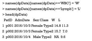
Renaming column would also facilitate the following data analysis and visualization in some cases. In the sample data, we simplify the names of WBC and Lymph variables into W and L, respectively.
Reshaping data frame between wide and long formats
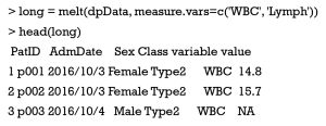
In R the measurements of different variables could be arranged into separate columns, which referred to as the “wide” format of data frame. Alternatively, all values of multiple variables could be stacked together into a single column (namely value column), for which an additional column is used for storing variable’s names (namely variable column); and this is the “long” format of data frame. Both melt() and dcast() functions in reshape2 package provide simple methods for converting between wide and long formats of data frame. In the sample data, two variables of WBC and Lymph are initially arranged as wide format, which could be converted into the long format.
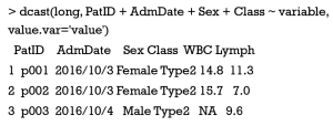
Subsequently, we could convert the long format back to wide format.
Merging two data frames
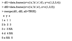
In R the merge() function is powerful for joining two data frames together based on the common variable(s). The missing value from one of the data frames could be flexibly treated, in which “NA” character will be filled if necessary. We construct two simple data frames for illustrating the merge() function.
Conclusions
Because R is extremely flexible for data manipulation, a number of methods could be likely employed for solving the same problem. However, such enhanced flexibility in usage would inevitably confuse the user, especially for these beginners. Therefore, we try to outline the common manipulations of data and then exemplify the typical applications in biological researches. Of course, only one method is recommended for a certain task in the present paper, which doesn’t mean that this method is absolutely superior to others. Because it is mainly intended to provide an overall landscape, both the arguments and usage for these introduced functions are not further described in details. Finally, any calculation or manipulation for our sample data has no biological meaning at all.
Acknowledgements
Funding: This work was supported by National Natural Science Foundation of China and Science and Technology Department of Sichuan Province, China (81300276 & 2015FZ0082).
Footnote
Conflicts of Interest: The authors have no conflicts of interest to declare.
References
- Ihaka R, Gentleman R. R. a language for data analysis and graphics. J Comput Graph Stat 1996;5:299-314.
- Tippmann S. Programming tools: Adventures with R. Nature 2015;517:109-10. [Crossref] [PubMed]

