
Use of the Cox regression analysis in thoracic surgical research
What is a survival analysis?
Introduction
Survival analysis refers to the statistical methods used for the analyzing of data where the outcome variable is the time until the occurrence of the event of interest. Survival analysis is also known as time to event analysis. Survival analysis applications are very large: For instance, they can be used for determining the survival rate of a population, or comparing the survival of two or more groups. Among them, Cox regression analysis is a very popular and widely-used method. Developed by David Cox in 1972 (1), its purpose is to evaluate simultaneously the effect of several factors on survival. Also known as proportional hazards model, its importance is crucial and has many applications in thoracic surgical research. This article describes the fundamental aspects of survival analysis (2) and of the Cox regression model in particular, and its application in a thoracic surgical research example.
Common terms
The event is the outcome of interest. The type of the event depends of the study purpose and must be clearly defined. Types of events include death, disease progression, relapse, recurrence, recovery…
The survival time is the time from the study starting point of the subject (time origin) to the occurrence of the event, or the date of the last contact. Time origin and event time must be clearly defined.
Only a subset of the subjects experiences the event. For the other subjects, the event is not observed. The survival time is then unknown and these observations are called censored.
Several types of censoring may be encountered:
- Right censoring is the most frequent form of censoring, and refers to the situation where the subject didn’t experience the event at his last time of observation (at the right side of the time line, cf. Figure 1). It can be encountered in two situations: the study ends before the subject experiences the event, or the subjects lefts the study during the study period (the subject is lost to follow-up), or withdraws from the study.
- In left censoring, the survival time of the subject is incomplete on the left side of his follow-up (at the left side of the time line), as the real entry date of the subject is unknown. It is rarely encountered.

Censoring must be distinguished from truncation, as no count of truncated observations is available. Truncation is due to sampling bias. The left-truncation is the most common form and is commonly happening in studies with delayed entry: only subjects who survived until the date of inclusion can be observed. The others are left-truncated, as the event of interest happened before the follow-up of the subjects starts. If the left-truncation is not taken into account, the event rate could be underestimated.
The Survival function represents the probability that a subject survives longer than a specified time t. It is expressed by S(t).
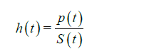
The hazard function, also referred to as the hazard rate, represents the probability that a subject who is under observation at a time t has an event at that time (for example, the risk of dying at time t). It is expressed by h(t) or λ(t). It corresponds to the ratio of the probability density function P(t) (the rate of death or failure events per unit time) and the survival function:
The hazard ratio (HR) is the estimate of the ratio of the hazard rate in the treatment group versus the hazard rate in the control group. The interpretation of the HR results is nevertheless similar to RR and OR: a HR higher than 1 means an increase in the hazard, an HR lower than 1 means a reduction the hazard, and a HR equal to 1 means there is no difference (effect) between the two groups. However, HR, RR and OR are estimates of different nature and should not be confused.
The interpretation of the HR is different depending whether the predictors are categorical or continuous. For categorical variables, a HR =2 for treatment group indicates that the hazard is 2 times higher that of control group. For continuous predictors, a HR =1.2 for example means a 20% increased hazard for each one-unit increase in the predictor.
Common survival analysis
Many techniques of survival analysis exist (2). We briefly list the most popular methods here:
- For the description of survival: the life table is the most basic form of survival analysis. Follow-up time is split into discrete time intervals. Number at risk represents the number of subjects remaining at observation at the beginning of a time interval, i.e., minus the number of censored subjects and the number of events occurred during the previous time interval. Surviving during the period between a survival time and the following survival time imply having survived until the beginning of this period and also surviving along this period. Estimate of survival is then obtained for each period by cumulatively multiplying the probabilities of surviving throughout each interval (using conditional probabilities properties). The most common method to define time interval is to consider the date of each event or censoring occurrence as the beginning of a new time interval (Kaplan-Meir process, see the Life table below) (Table 1). Another method relies on using intervals of time of the equal length (Actuarial method);
- For generating survival curve of a group of subjects: Kaplan-Meier estimator (3). An example of this non-parametric method is briefly presented below;
- For the comparison of the survival times of two or more groups: the log-rank test (4);
- For the analysis of the effect of categorical or quantitative variables on survival, Cox regression is the most used method.

Full table
What is Cox regression?
Cox regression model is also currently known as Proportional hazards model. It is a semi-parametric survival model, and a regression method. Regression is a statistical technique investigating the relationship between a dependent variable and explanatory variables, also known as covariates, independent variables or predictors. Therefore, Cox regression permits to evaluate simultaneously the effect of several factors (adjusted comparisons) on survival. Univariate and multivariate models can be performed. It is formulated as follows:
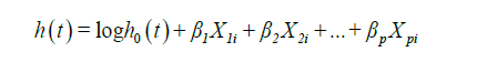
Where:
- t is the survival time;
- h(t) is the hazard function, determined by a set of p independent variables X1i, X2i, .., Xpi for i subjects;
- β1, β2, .., βp are the coefficients (also called parameters) which quantify the statistical relationship between the p covariates and the survival (regression coefficients);
- h0 is the baseline hazard. It corresponds to the value of the hazard if all the Xi are equal to zero.
Methods
Many statistical software programs can be used to perform a Cox model: SPSS, SAS, Stata, R… The present example was performed with R and the package “survival” (5,6).
A dataset of 601 patients who underwent lung cancer surgery was used for illustration. The 3-year overall survival after surgery was analyzed, and different factors potentially associated with a higher risk of death were tested. Overall 3-year survival was 67%.
Kaplan-Meier curves and log-rank test
Kaplan-Meier is used to estimate the survival function. The following curves respectively show the overall 3-year survival (Figure 2) and survival in two age-groups (age above 70, and age equal or less than 70) in Figure 3. The two groups were compared with a log-rank test, and the difference between the two survival curves was statistically significant (P=0.0077), meaning that survival differ significantly between the subjects aged of 70 or less and the subject older than 70. Number of patients at risk represents the number of patients still under observation at the considered time interval. The curves are presented here with their optional 95% confidence band. Note that the interpretation of curves is not valid when the number of subjects is very low.


Which variables are needed for Cox regression, and how must they be coded?
The event variable must be coded as a binary variable 1: event (also referred as failure)/0: no event (i.e., right-censored). Here, the definition of an event is death. Observations with an unknown censor value are considered as missing, and the subjects are removed from the analysis.
The survival time variable is a continuous variable. In our example, it is the time from surgery to the event (here death) or the censoring.
The predictors can be categorical or continuous.
Which method should be used?
In the exact method, the exact probability of all possible orderings of events is calculated. It is the most computing time-consuming method. Two approximations to the exact method have been developed to provide faster results: Breslow and Efron methods. While popular and the default method of many software programs, the Breslow approximation has shown to be less accurate than Efron method in many situations. The Efron approximation is generally the recommended method.
Interpretation of the Cox regression results
Here, a multivariate Cox model was performed to describe the risk factors associated with a lower 3-year survival. Age, gender, simplified cancer stage, decortication procedure, neoadjuvant therapy and forced expiratory volume in 1 second (FEV1) were included in the model. The results are presented below (Table 2).

Full table
The results can be interpreted as follows:
The regression coefficients: a positive regression coefficient indicates an increased hazard of death, and a negative regression coefficient indicates a lower hazard. In our example, the regression coefficients of age >70, Female gender, decortication, stages >1, and neoadjuvant therapy are positive, and the regression coefficient of FEV1 ≥80 is negative.
The regression coefficients are always presented with their standard error (SE): SE is the measure of the uncertainty of the regression coefficient.
The HR: HR is obtained from the exponential of regression coefficient, and gives the effect size of the predictors. In our example, age variable has a HR =1.793. It means that the hazard (here the risk of death) in the group of patients above 70, is about 1.8 times higher than in the group of patients under 70.
However, in order to conclude we also need to check the statistical significance. We have to look at the confidence intervals of the HRs, and the probability values (P value).
A 95% confidence interval (95% CI) means that if the estimation process was repeated infinite times, then 95% of the calculated intervals would contain the true parameter value. Here, lower and upper 95% CIs of the HR are shown. If the value 1 is not contained in the interval, then the association between survival and the tested variable is statistically significant.
The level of significance is set before the beginning of the statistical analysis (and commonly set at 0.05). When the P value is lower than this threshold, the null-hypothesis of no difference in survival between groups can be rejected. In our example, the significance level was set at 0.05. Age above 70, decortication and pathological stages were significantly associated with survival according to P value and 95% CI. Female gender, FEV1 equal above 80 and neoadjuvant therapy variables both were related to a P value higher than 0.05. Moreover, and not surprisingly, HR 95% CIs of both variables included 1. These variables are not significantly associated with survival. Therefore we can’t conclude on these variables.
Finally, we can conclude that in our model, age above 70, simplified cancer stage above 1 and decortication are significantly associated with an increased hazard of death.
What to verify?
Our model is only valid if we respect following conditions:
Proportional hazards assumption
The assumption of a constant relationship between the dependent variable and the explanatory variables: in other words, each HR is assumed to be constant over time. This is called the proportional hazards assumption. In a comparison between two groups, we can graphically evaluate it with Kaplan-Meier curves and log-log plots. If the two survival curves remain parallel and don’t intersect, we can assume in a first approach the proportional hazard. In a multivariate model, we can check the proportional hazards assumption for each covariate with the following methods (7):


Full table
If a covariate violates the proportional hazards assumption, several solutions can be applied:
- Stratify on this covariate: then there won’t be any estimation of HR for this variable;
- Add an interaction between the covariate and time.
Log-linearity
The relationship between continuous variables and survival is assumed to be linear. If continuous predictors are included in the model, this assumption must be checked. Plotting the residuals is a method for graphically detecting non-linearity (residuals are computed from the observed values minus estimated values).
Conclusions
In this article, we focused on the basics of survival analysis and Cox regression, which are routinely used in thoracic surgery research. We insisted on the Cox model assumptions checks, which is a crucial part of Cox analysis and shouldn’t be neglected.
We didn’t address however the advanced methods of Cox regression. We can cite here the handling of time-dependent covariates (8), which may be encountered in thoracic surgery research. A covariate is considered as time-dependent or time-varying when its values change over time of follow-up. Several methods allow incorporating these variables in a Cox model, including counting process. In these methods, a dataset including multiple rows for each subject is used, with each row corresponding to an interval of time where the time-dependent variable remains constant.
Other Cox models extensions can also be cited, such as frailty models for non-independent data, or competing risks models in the case of several simultaneous events.
Acknowledgements
None.
Footnote
Conflicts of Interest: The authors have no conflicts of interest to declare.
References
- Cox DR. Regression Models and Life-Tables. J R Stat Soc Ser B (Methodol) 1972;34:187-220.
- Clark TG, Bradburn MJ, Love SB, Altman DG. Survival analysis part I: basic concepts and first analyses. Br J Cancer 2003;89:232-8. [Crossref] [PubMed]
- Kaplan EL, Meier P. Nonparametric Estimation from Incomplete Observations. J Am Stat Assoc 1958;53:457-81. [Crossref]
- Bland JM, Altman DG. The logrank test. BMJ 2004;328:1073. [Crossref] [PubMed]
- Therneau T. A Package for Survival Analysis in S. version 2.38. 2015. Available online: (last accessed march 2018).https://CRAN.R-project.org/package=survival
- Fox J, Weisberg S. Cox Proportional-Hazards Regression for Survival Data in R. An Appendix to An R Companion to Applied Regression, Second Edition. 2011 Feb 23. Available online: (last accessed march 2018).https://socialsciences.mcmaster.ca/jfox/Books/Companion/appendix/Appendix-Cox-Regression.pdf
- Grambsch PM, Therneau TM. Proportional hazards tests and diagnostics based on weighted residuals. Biometrika 1994;81:515-26. [Crossref]
- Fisher LD, Lin DY. Time-dependent covariates in the Cox proportional-hazards regression model. Annu Rev Public Health 1999;20:145-57. [Crossref] [PubMed]

